First Step of Linux and Root
本文最后更新于 2026年1月24日
Lesson 0 install root and software on your compute
If you get the THU’s computer cluster account, use following commands to get into.
$ ssh -XY -p 48571 -o ServerAliveInterval=5 yourname@hepthu.comYou can also run code on your pc if you have installed root, it’s up to you.
homebrew Click this link to go to the Homebrew page, follow the instructions to install Homebrew on your Mac. Homebrew is a software package manager that allows you to download many applications on your Mac!
After finishing the installation, paste the following command in a macOS terminal to install CERN ROOT software: $ brew install root. This way, you can also install applications like firefox which you can’t find in the App Store.
Additionally, $ indicates a shell command, so drop the $ sign when you copy the command.
Lesson 1 base commands for Linux
Some simple commands you can have a try!
1 | |
Vim editor
1 | |
you will use the next commands from time to time
vi somefile -> press i into edit mode -> do something ->esc exit edit mode -> :wq
Some tricks that can help you:
Press the TAB key to automatically complete some of your commands, such as file names. Pressing it twice will show you the available commands/file names you can input.
Press ↑ to retrieve previous commands.
Lesson 2 root 基础练习
进入root环境
$ root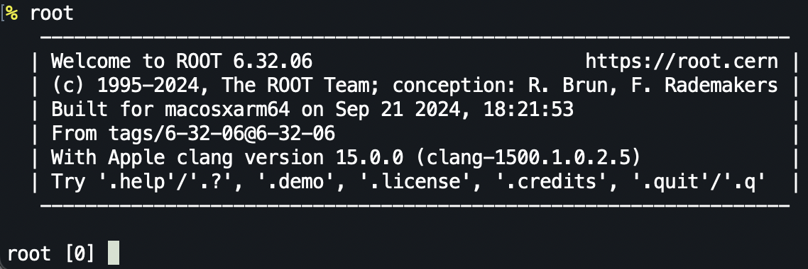
root [0] .q 退出root
root能输入一句解释一句
也可以边解释边执行或者编译后执行一个程序文件,用root yourprogram.C
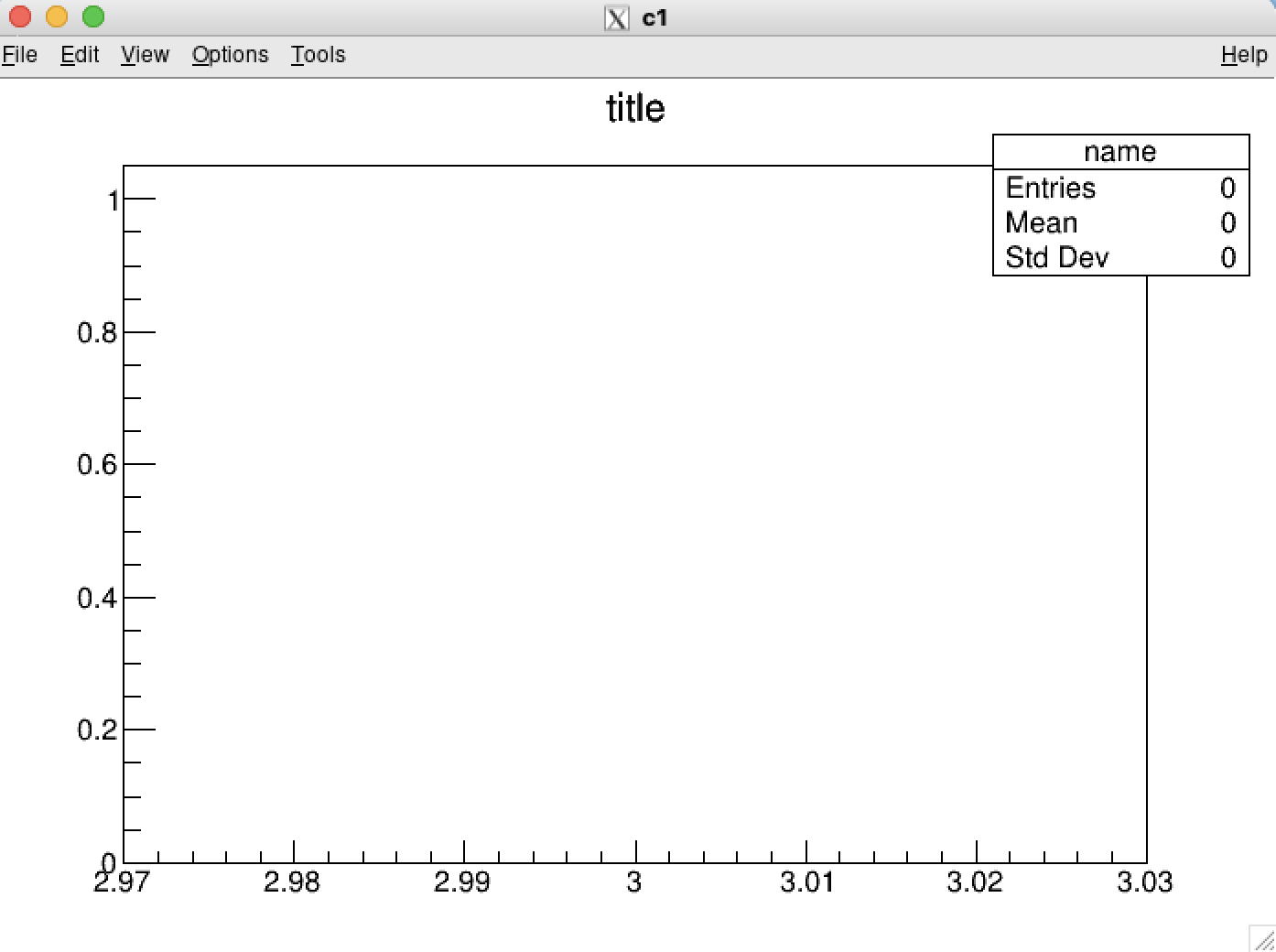
例如:可以在root中输入下面的程序用来创建一个空白的直方图TH1F* graph=new TH1F("name","title",200,2.97,3.03);graph->Draw();
但一个空白的直方图是很无趣的,你还需要用Fill来填入数据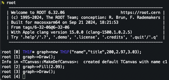
此外我们还能直接创建一个程序文件,以放入更长的程序
Get start!
$ vi test.C
//push i to enter the insert mode//
1 | |
//push ESC to end the insert mode//
:wq //save and exit
$ root test.C //run your code
///successful!///
.q //exit the program
Let’s add something into your graph!
1 | |
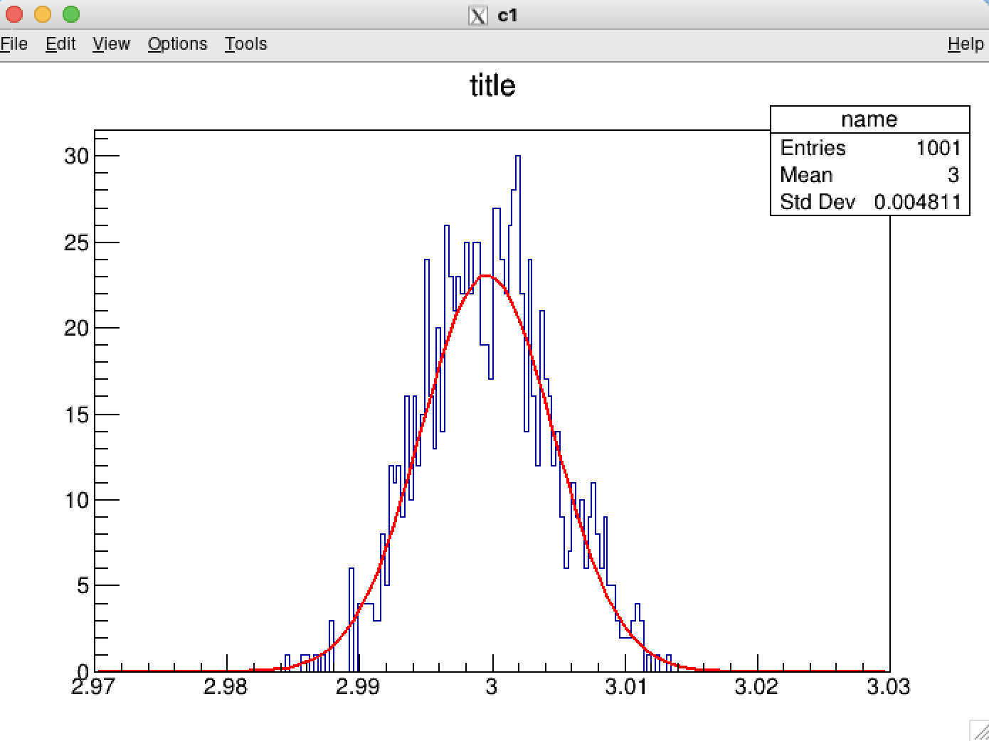
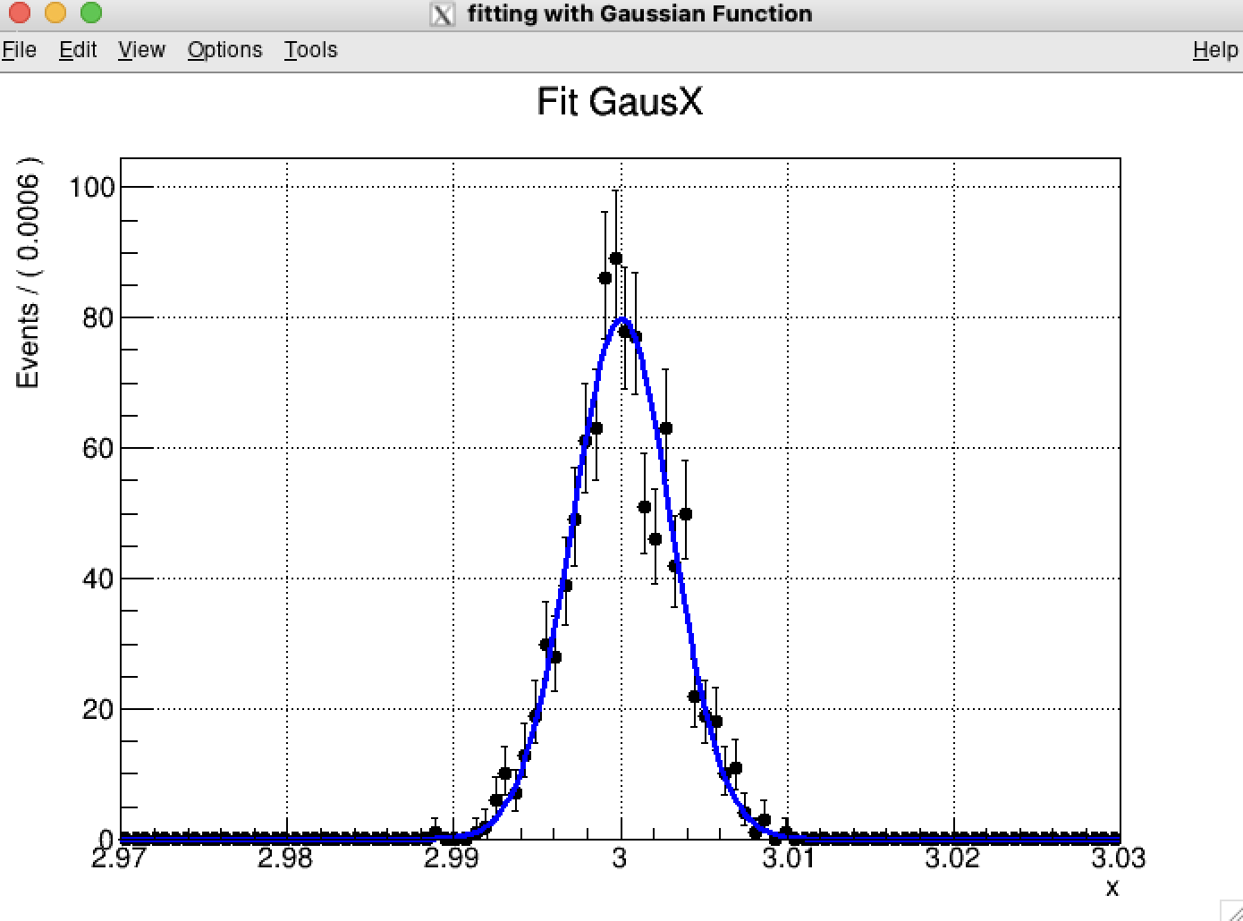
Wow! now you can use root to do some simple fit works. but we usually use RooFit to do more complex job! So, ready for more programs!
以上只是一些基础的拟合,很多参数我们并不能自己去定义,没有灵活性,RooFit中则提供了更加专业的拟合函数。
Lesson 2 Gaussian fitting using RooFit
1 | |
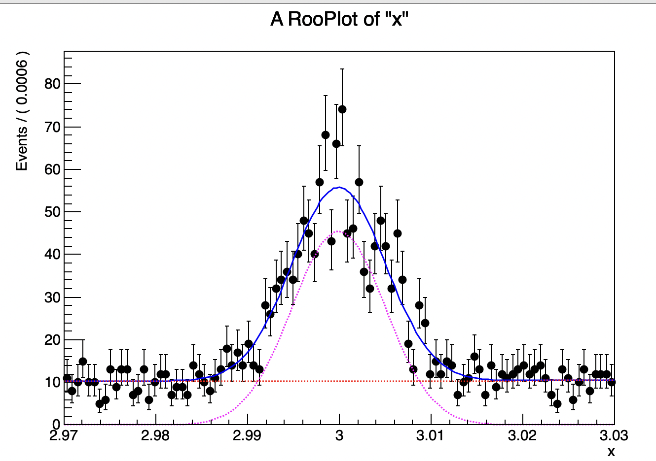
一个函数看起来有些孤单,我们可以用RooAddPdf这个函数把两个函数放在一起
RooRealVar fsig(“fsig”,”fsig”,0.2,0,1.);
//model(x) = fsig*gaus(x) + (1-fsig)*chev(x)
RooAddPdf model(“fsig”,”fsig”,RooArgList(gaus,chev),fsig);
1 | |
以上是一维拟合,但很多时候我们会研究两个不同组分,这样就需要进行二维拟合。二维拟合就不单单是把两个PDF加和在一起了,而是需要乘积,可以理解为同时出现两个组分的概率。举例来说,对于x事件,他有发生和不发生两个概率设为p(x) q(x),对于y事件同样的p(y) q(y),那么对于所有的事件就有四种情况,这四种情况的概率相对应的就是p(x)*p(y) 是x,y同时发生的概率,其他的相同。所以我们需要构建四个概率函数来表示对于这两个事件不同组合的各种情况出现的概率。
Note: 默认的随机生成的种子号是0,一般会根据时间设置种子号,这样每次生成都是不一样的,但是这里可能是为了调试的方便,让种子号为0时是一个确定的值,所以如果你的程序跟我一样的话生成的数据也是一模一样的,并不是那么随机。你可以RooRandom::randomGenerator()->SetSeed(seed)来自定义种子号,还有另外一种方式gRandom->SetSeed(seed),前者是对RooFit中的随机数生成器进行设置,RooFit中的一些需要随机数的函数都会依赖这个值,后者是面向ROOT的全局随机数生成器,当除RooFit之外的其他库中也需要随机数生成的时候,会依赖这个seed。简单来说,后者可以包含前者,你可以使用gRandom->GetSeed()去查看当前的seed。
1 | |
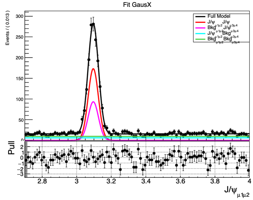
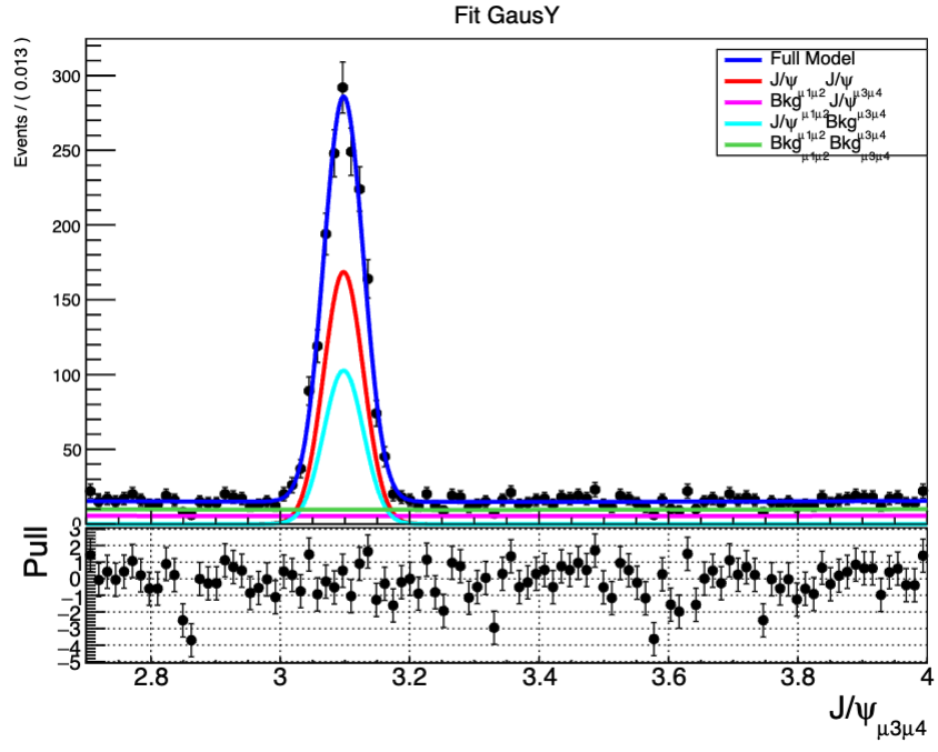
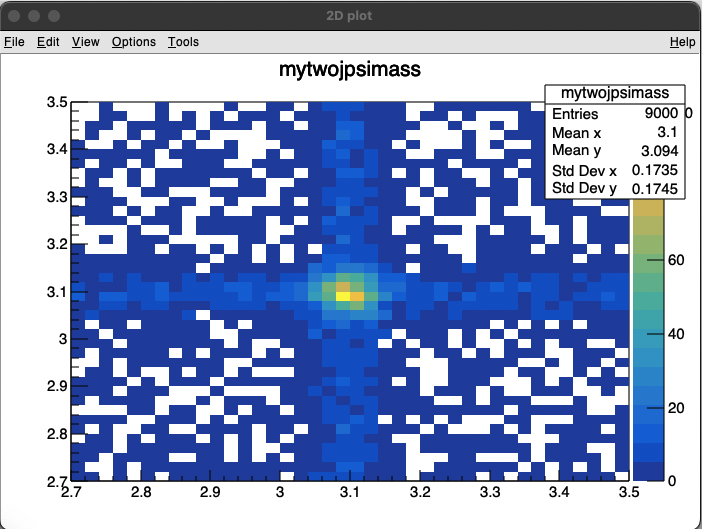
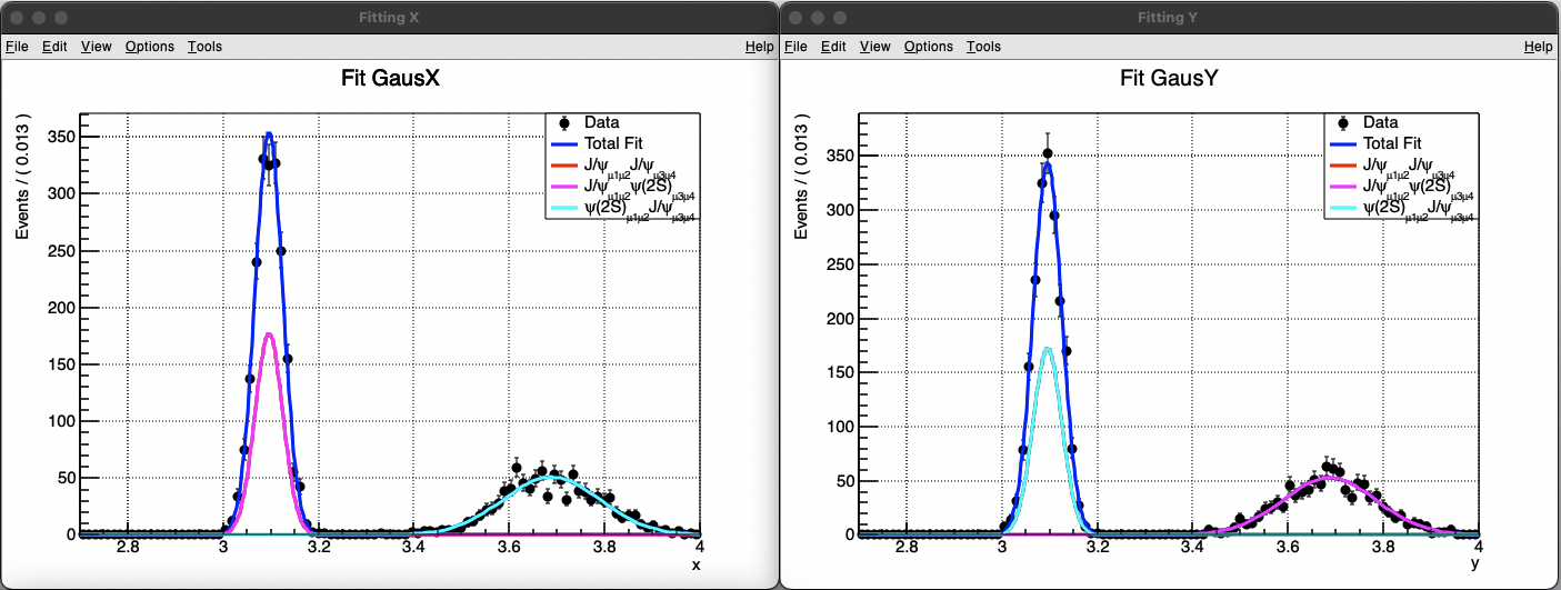
Lesson 3 2D fitting
下面展示了两个二维拟合
1 | |

1 | |
Lesson 3+ Pull Plot
当我们想看拟合曲线和数据点之间拟合是否拟合得很好的话,就需要看pull分布,就相当于将拟合曲线拉直看数据点相对于曲线的距离,下面是对于xframe的pull图,对应的
1 | |